[논문 리뷰] SIREN
![[논문 리뷰] SIREN](/assets/SIREN/cameramen_256.png)
논문 리뷰
Implicit Neural Representations with Periodic Activation Functions (SIREN)
Vincent Sitzmann, 2020
=================================================================
이번에는 Implicit Neural Representations (INR)에 관한 논문을 리뷰하고자 합니다. 그리고 공개된 코드를 기반으로 실험을 진행하고 내용을 정리하고자 합니다.
(이 논문은 너무 길고 수식이 많아 이해하는 데 어려움도 많고 잘 정리할 자신이 없어 최대한 간략히 작성하고 여러 자료를 읽으며 INR에 대해 이해한 바대로 정리하겠습니다.)
Implicit Neural Representations (INR)
본 논문에서는 Implicit Neural Representation (INR)을 학습하는 데 있어, Activation 을 Periodic 한 성질을 가지는 함수(ex. sin 함수)를 사용하는 것이 더 성능이 좋다는 것을 주장합니다. 그럼 INR이 어떤 내용인지를 먼저 알아볼 필요가 있습니다.
INR 은 데이터를 Nueral Network 를 통해 Continuous 한 좌표 값으로 매핑시켜 하나의 함수로 작동하도록 표현합니다. 이러한 특설을 활용해 다양한 분야에서 사용되는 것으로 파악됩니다. 먼저, 최근 각광 받고 있는 분야로 이미지 혹은 3D 데이터에서 새로운 각도의 데이터를 생성하는 NeRF가 있습니다. 이미지를 더 높은 품질로 향상시키는 Super resolution 분야에서도 많이 사용되고 있습니다. 그리고 데이터를 압축 전송하는 방법으로도 사용되고 있습니다. INR 모델로는 MLP 가 사용되는 데, 그 모델을 Quantization, pruning 을 거쳐 모델의 크기를 줄이면 데이터를 송신하는 단에서는 MLP 모델만 전송하고 수신하는 기기에서 받은 MLP 모델을 통해 좌표 값을 넣어 Feed Forward 연산을 수행하면 기존의 데이터를 복원할 수 있습니다.
본 논문에서 공개한 코드를 기반으로 INR 이 어떻게 학습되고 작동하는 지 간략히 정리하자면 아래와 같습니다. 데이터는 100x100 크기의 흑백 이미지라고 가정하고 설명하겠습니다.
- 데이터의 크기에 따라 좌표를 Continuous 한 값, [-1, 1] 으로 표현. 이러면 좌표 (-0.5, 0) 은 이미지 픽셀에서 (25, 50) 위치의 픽셀 값이 될 것입니다.
- MLP 모델 생성. 본 논문에서는 3개의 Linear layer 사용
- 모든 데이터 (좌표, 픽셀)를 하나의 Batch로 구성
- 좌표를 입력으로, 픽셀을 Ground truth 로 MSE Loss 를 활용해 학습
- (추론) [-1, 1] 사이의 값으로 원하는 크기만큼 구간을 나누어 좌표를 생성하여 학습한 모델을 통해 이미지 복원
INR의 작동 과정에 대해 이제 코드와 함께 정리해보도록 하겠습니다.
1. Continuous 한 좌표 값 생성
def get_mgrid(sidelen, dim=2):
    '''Generates a flattened grid of (x,y,...) coordinates in a range of -1 to 1.
    sidelen: int
    dim: int'''
    tensors = tuple(dim * [torch.linspace(-1, 1, steps=sidelen)])
    mgrid = torch.stack(torch.meshgrid(*tensors), dim=-1)
    mgrid = mgrid.reshape(-1, dim)
    return mgrid
위 함수의 인자 값 sidelen 은 이미지의 크기를 나타냅니다. 그리고 이미지의 크기를 정사각형 모양의 데이터로 가정했기에 하나만 받도록 했습니다. 그리고 dim 은 이미지의 차원(혹은 축의 개수)을 나타내는 데, 흑백 사진을 사용하니 x축, y축 2개의 차원을 사용합니다.
2. MLP 모델 생성
# Define Model
class SineLayer(nn.Module):
    def __init__(self, in_features, out_features, bias=True,
                 is_first=False, omega_0=0):
        super().__init__()
        self.omega_0 = omega_0
        self.is_first = is_first
        self.in_features = in_features
        self.out_features = out_features

        self.linear = nn.Linear(in_features, out_features, bias=bias)

        self.init_weights()

    def init_weights(self):
        with torch.no_grad():
            if self.is_first:
                """
                # 본 논문에서 첫 번째와 나머지 layer 의 weights 을 아래와 같이 설정하는 것이 가장 좋았다고 합니다.
                # 첫 번째 layer 를 제외하고는 +- sqrt(c/n) 사이로 초기화 하는 것이 sin을 적용했을 때 uniform 분포를 따르는 것을 보장할 수 있다고 합니다.
                # omega_0 로 sine 함수 정의에 의한 것인데, 자세한 내용은 논문을 참고하시길 바랍니다.
                """
                self.linear.weight.uniform_(-1 / self.in_features,
                                            1 / self.in_features)
            else:
                self.linear.weight.uniform_(-np.sqrt(6 / self.in_features) / self.omega_0,
                                            np.sqrt(6 / self.in_features) / self.omega_0)

    def forward(self, x):
        return torch.sin(self.omega_0 * self.linear(x))

    def forward_with_intermediate(self, x):
        # For visualization of activation distributions
        intermediate = self.omega_0 * self.linear(input)
        return torch.sin(intermediate), intermediate

class Siren(nn.Module):
    def __init__(self, in_features, hidden_features, hidden_layers, out_features, outermost_linear=False,
                 first_omega_0=30, hidden_omega_0=30.):
        super().__init__()
        net = []
        net += [SineLayer(in_features, hidden_features, is_first=True, omega_0=first_omega_0)]
        for i in range(hidden_layers):
            net += [SineLayer(hidden_features, hidden_features, is_first=False, omega_0=hidden_omega_0)]
        if outermost_linear:
            final_linear = nn.Linear(hidden_features, out_features)

            with torch.no_grad():
                final_linear.weight.uniform_(-np.sqrt(6 / hidden_features) / hidden_omega_0,
                                              np.sqrt(6 / hidden_features) / hidden_omega_0)
            net += [final_linear]
        else:
            net += [SineLayer(hidden_features, out_features, is_first=False, omega_0=hidden_omega_0)]

        self.net = nn.Sequential(*net)

    def forward(self, coords):
        coords = coords.clone().detach().requires_grad_(True) # allows to take derivatives
        output = self.net(coords)
        return output, coords

    def forward_with_activations(self, coords, retain_grad=False):
        """
        Returns not only model output, but also intermediate activations,
        Used for visualizing
        """
        activations = OrderedDict()
        activation_count = 0
        x = coords.clone().detach().requires_grad_(True)
        activations['input'] = x
        for i, layer in enumerate(self.net):
            if isinstance(layer, SineLayer):
                x, intermed = layer.forward_with_intermediate(x)
                if retain_grad:
                    x.retain_grad()
                    intermed.retain_grad()
                activations['_'.join(str(layer.__class__), "%d" % activation_count)] = intermed
                activation_count += 1
            else:
                x = layer(x)
                if retain_grad:
                    x.retain_grad()
            activations['_'.join(str(layer.__class__), "%d" % activation_count)]
            activation_count += 1
        return activations
model = Siren(in_features=2, hidden_features=256, hidden_layers=3, out_features=1, outermost_linear=True)
model.cuda()
본 논문에서 주된 contribution 을 반영한 모델입니다. 기본적으로 Linear layers 로 이루어진 MLP 이지만, activation 함수로 sine 함수가 사용되었습니다. 그리고 Sine 함수를 사용함으로써 사용되는 가중치 초기화 방법에 대해 소개했는 데 위의 코드에 간략히 적어놓았습니다.
3.모든 데이터 (좌표, 픽셀)를 하나의 Batch로 구성
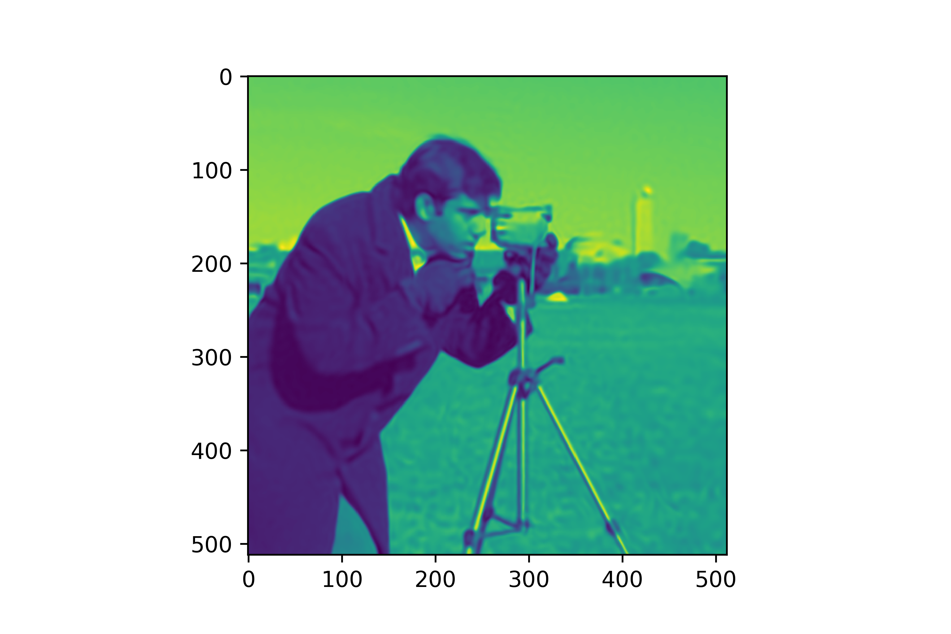
def get_cameraman_tensor(sidelength):
    img = Image.fromarray(skimage.data.camera())
    transform = Compose([
        Resize(sidelength),
        ToTensor(),
        Normalize(torch.Tensor([0.5]), torch.Tensor([0.5]))
    ])
    img = transform(img)
    return img

class ImageFitting(Dataset):
    def __init__(self, sidelength):
        super().__init__()
        img = get_cameraman_tensor(sidelength)
        self.pixels = img.permute(1, 2, 0).view(-1, 1)
        self.coords = get_mgrid(sidelength, 2)

    def __len__(self):
        return 1

    def __getitem__(self, idx):
        if idx > 0: raise IndexError

        return self.coords, self.pixels

sidelength = 256
cameramen_dataset = ImageFitting(sidelength)
dataloader = DataLoader(cameramen_dataset,
                        batch_size=1,
                        pin_memory=True,
                        num_workers=0)
데이터는 논문에서 사용된 cameraman 이미지 데이터가 사용되었습니다. 위의 코드에서 보이는 바와 같이 모든 좌표와 픽셀 값을 하나의 Batch 로 구성하는 것을 알 수 있습니다. ( 이렇게 되면 back-propagation 과정에서 GPU 메모리가 상당히 많이 사용되는데, mini-batch 로 나누어서 학습시키면 성능 차이가 있는 지 나중에 확인해봐야겠습니다.)
4. 좌표를 입력으로, 픽셀을 Ground truth 로 MSE Loss 를 활용해 학습
total_steps = 500
steps_til_summary = 100
optim = torch.optim.Adam(model.parameters(), lr=1e-4)
model_input, ground_truth = next(iter(dataloader))
model_input, ground_truth = model_input.cuda(), ground_truth.cuda()

for step in range(total_steps):
    model_output, coords = model(model_input)
    loss = ((model_output - ground_truth)**2).mean()

    if not step % steps_til_summary:
        print(f'Step [{step:3d}/{total_steps:3d}], Loss {loss.item():.4f}')
        img_grad = gradient(model_output, coords)
        img_laplacian = laplace(model_output, coords)

        fig, axes = plt.subplots(1, 3, figsize=(18, 6))
        axes[0].imshow(model_output.cpu().view(sidelength, sidelength).detach().numpy())
        axes[1].imshow(img_grad.norm(dim=-1).cpu().view(sidelength, sidelength).detach().numpy())
        axes[2].imshow(img_laplacian.cpu().view(sidelength, sidelength).detach().numpy())
        plt.show()
    optim.zero_grad()
    loss.backward()
    optim.step()
학습과정은 일반적인 DNN 학습 과정과 동일합니다. 다만, epoch 가 제외되어 있고, Validation 과정이 없습니다. (적어보니 일반적인 학습 과정과 다르네요;;) optimizer 는 Adam 을 사용했고, 500 step 만큼 학습시킵니다.
5. 추론 Super Resolution
사실 이제 좌표 값을 넣고 원래 이미지를 잘 복원하는 지 확인하면 됩니다. 추가적으로 개인적으로 Super Resolution 으로 어떻게 활용될 수 있는지도 실험해보았는 데 관련 내용으로 설명드리겠습니다.
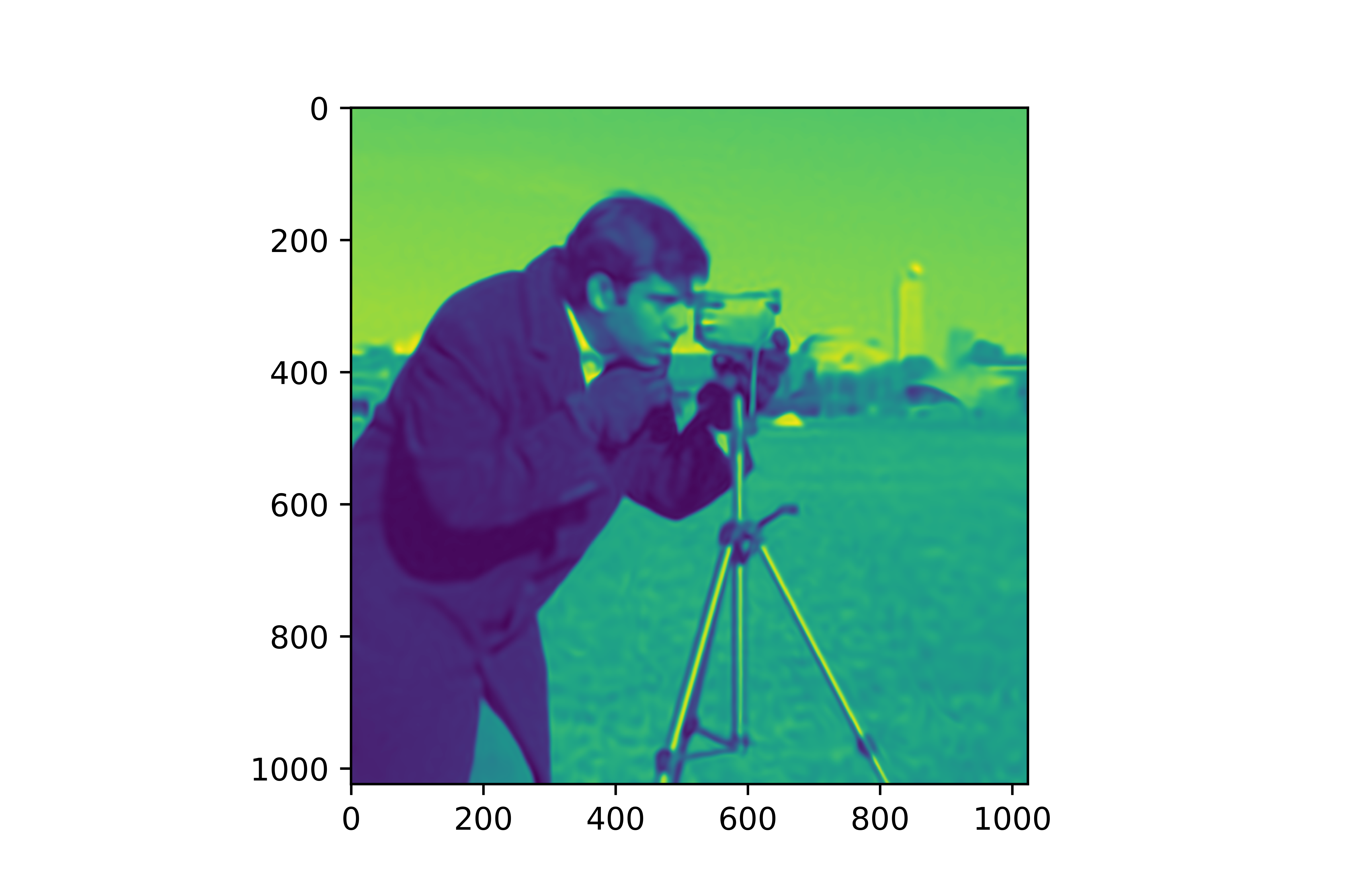
SR_sidelength = 1024
SR_coords = get_mgrid(SR_sidelength)
model.eval()
SR_model_output, _ = model(SR_coords.cuda())
plt.imshow(SR_model_output.cpu().view(SR_sidelength, SR_sidelength).detach().numpy())
plt.show()
Super Resolution 은 결국 이미지에서 각 픽셀 사이에 추가되는 픽셀 값을 추정하는 것 입니다. 흑백 이미지에서 (1, 2)위치에 있는 픽셀과 (1, 3) 사이의 픽셀 값이 무엇인지를 추정해야하는 데, 여기사 말하는 (1,2)와 (1,3)은 위치로 (좌표가 아니라) discrete 합니다. 하지만 INR 에서는 이 위치를 좌표(coordinate)으로 표시합니다. 그리고 우리는 이미지의 길이 256 을 [-1, 1] 사이의 값으로 256 등분하여 나누어 표현했습니다. 따라서, 각 좌표를 실수로 표현할 수 있습니다. 즉, (0.5, -0.3792) 란 위치는 존재할 수 없지만 좌표는 존재할 수 있습니다. 따라서, [-1, 1] 사이의 값을 원하는 크기만큼 등분하여 좌표를 구하고 Feed-Forward 를 진행하는 방식으로 Super Resolution 을 수행할 수 있습니다.
위의 예제는 학습 시에는 256 x 256 크기의 이미지를 1024 x 1024 크기로 해상도를 키우고 싶을 때의 예시입니다.
그리고 아래의 세 사진은 원본 이미지와 512로 SR을 진행했을 때, 1024로 SR을 진행했을 때의 결과입니다.
나의 의견
Implicit neural representation 에 대한 대략적인 내용과 그 방법에 대해 SIREN 논문을 통해 처음 알게되었습니다. MLP 모델을 하나의 데이터에 overfitting 시킨다는 것인데, overfitting은 항상 방지해야 돼! 라고 단정지었는 데, 이런 생각을 깨게 되네요. Continuous 한 좌표 값을 통해 새로운 각도의 이미지를 생성한다던지, 3D 데이터 등 용량이 큰 데이터를 MLP 모델 하나로 압축하여 전송한다던지 활용할 수 있는 방안이 많은 연구인 것 같습니다.
Reference
논문 : https://arxiv.org/abs/2006.09661 Github : https://github.com/vsitzmann/siren